Adaptive Inference for Medical Vision Transformers:
Token Reduction or Early Exit?

Why Adaptive Inference for Medical Vision Transformers?

Vision Transformers (ViTs) have achieved state-of-the-art results across medical imaging tasks such as dermatological lesion classification, chest X-ray diagnosis, histopathological analysis, and ophthalmic imaging. Yet their high computational cost creates critical barriers for clinical deployment:

Two prominent efficiency strategies exist: Token Reduction (TR) prunes spatially redundant patches, and Early Exiting (EE) terminates inference when prediction confidence is sufficient. Prior work treats these in isolation. We ask: which strategy is right for which dataset and for which sample?

Through comprehensive dataset profiling, we show that optimal strategies vary dramatically across modalities, and that adaptively combining TR and EE yields gains neither can achieve alone.

A Three-Stage Adaptive Inference Framework

Our framework fine-tunes DeiT-S with early exit heads, profiles each dataset's redundancy and complexity characteristics, then deploys a unified inference pipeline that dynamically selects the optimal path per sample at test time.

Stage 1: Multi-Exit Loss

We attach lightweight two-layer MLP classifiers (with layer normalization) to the CLS token at layers 4, 7, and 10 of DeiT-S. All heads are trained jointly:

where $w_4 = w_7 = w_{10} = 0.3$ and $w_\text{final} = 1.0$.

Stage 2: Spatial Redundancy Profiling via JSD

For each validation sample, we compute a ground-truth redundancy score from attention distributions:

High $y_\text{red}$ (close to 1) indicates low divergence between attention patterns — i.e., the image is spatially redundant and tokens can be safely pruned. A lightweight CNN is then trained to predict $\hat{y}_\text{red}$ directly from input pixels, avoiding full forward passes at test time.

📊 Figure 1: Add static/fig1.png from the paper — token-level redundancy profiles and sample complexity analysis.

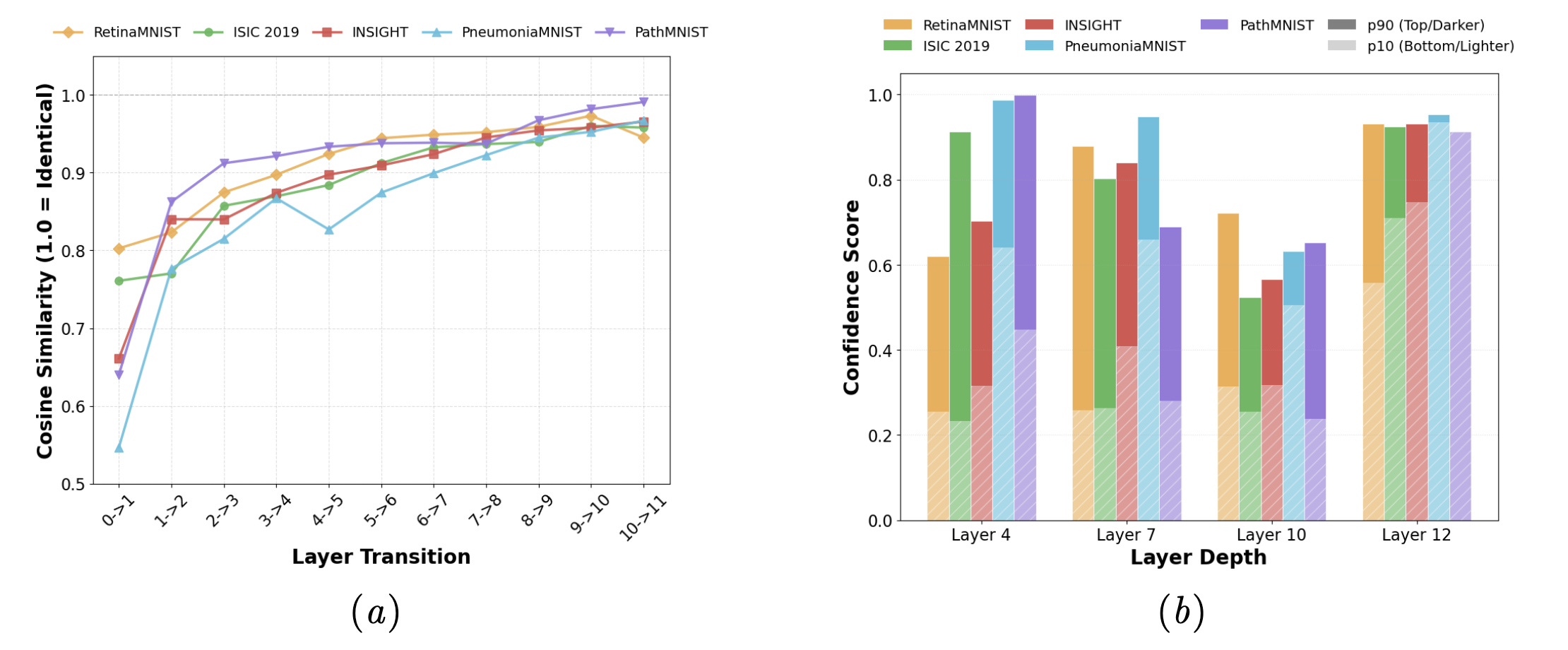
Figure 1. Dataset redundancy and complexity analysis across DeiT-S layers. (a) Token-level cosine similarity across layer transitions — RetinaMNIST and ISIC2019 exhibit high initial similarity (~0.8), while INSIGHT, PathMNIST, and PneumoniaMNIST start lower (~0.6). All datasets show monotonically increasing similarity. (b) Sample-wise confidence at EE checkpoints (layers 4, 7, 10, 12) for easy samples (90th pct, lighter) and hard samples (10th pct, darker). PathMNIST and PneumoniaMNIST achieve high early confidence; RetinaMNIST and INSIGHT maintain persistent easy-hard gaps, requiring deeper inference.

Stage 3: Unified Inference Pipeline

At test time, for each input image $\mathbf{x}$:

1. Score Predictor estimates $\hat{y}_\text{red}$; set use_tr = (ŷ_red > θ_R)
2. Process ViT layer-by-layer through 12 transformer blocks
3. At each checkpoint (layers 4, 7, 10): if $c_k > \theta_\text{EE}$ → exit and return prediction; else if TR active → prune tokens before next block
4. If no early exit, use final layer 12 head

This pipeline ensures: spatially redundant samples use TR → high-confidence samples exit early → complex samples receive full computation.

Superior Efficiency–Accuracy Trade-offs

We evaluate on five medical imaging datasets: ISIC2019 (skin lesions, 9-class), PathMNIST (colon tissue, 9-class), PneumoniaMNIST (pneumonia, binary), RetinaMNIST (diabetic retinopathy, 5-class), and INSIGHT (cataract, real-world clinical data, 4-class).

Unified Framework Performance

Computation Cost Analysis

Visualizations

🖼️ Figure 4: Add static/fig4.png — token reduction visualization on INSIGHT (cataract) and PathMNIST samples.

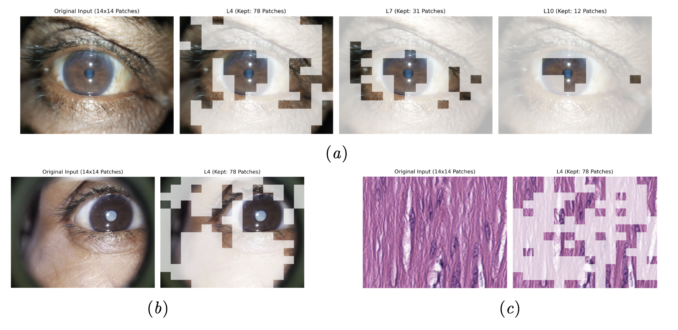
Figure 4. Visualization of adaptive framework behavior on INSIGHT and PathMNIST samples. (a) TR-only path: sequential token reduction at 40% keep rate across all checkpoints, preserving informative pupil regions through layer 12. (b)–(c) Combined TR+EE examples: TR activates at the first checkpoint, followed by early exit — clear cataract evidence or salient tissue structure enables confident prediction without deeper layers.

📈 Figure 3: Add static/fig3.png — token reduction strategy comparison (Top-K, EViT, Random, ToMe) across PathMNIST and INSIGHT.

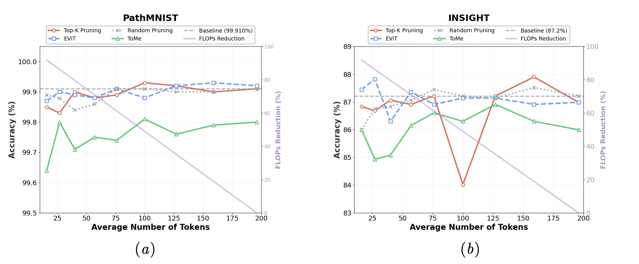
Figure 3. Token reduction strategy comparison across medical imaging datasets. PathMNIST (left) tolerates aggressive reduction — all strategies maintain >99.7% accuracy at 40 tokens. INSIGHT (right) shows greater sensitivity; EViT proves most stable, maintaining 86.3% at 40 tokens (−0.9pp). ToMe collapses below 76 tokens on INSIGHT.

Cite This Work

If this work is useful in your research, please cite:

@inproceedings{byun2026adaptive,
  title     = {Adaptive Inference for Medical Vision Transformers:
               Token Reduction or Early Exit?},
  author    = {Byun, Ji Young and Lee, HyunSeo and Shuff, Jordan and
               Venkatesh, Rengaraj and Shekhawat, Nakul S. and
               Parikh, Kunal S. and Chellappa, Rama},
  booktitle = {Medical Imaging with Deep Learning (MIDL)},
  year      = {2026}
}